The Blueprint of Waves: Understanding Periodic Waveforms in Engineering

Introduction

In the world of engineering, signals and waves are everywhere,  from the hum of alternating current in power lines to the data streams driving modern communication systems. At the heart of many of these phenomena lies the concept of periodic waveforms, the rhythmic, repeating signals that serve as the backbone of countless technologies. Understanding these waveforms is not just an academic exercise; it is a practical necessity for engineers designing systems that need to manage, analyze, and transmit information efficiently.

Periodic waveforms,  such as sine, square, and triangular waves  are the building blocks of signal processing and electronics. They are defined by their predictable repetition over time, a property that allows engineers to model, manipulate, and optimize them for real-world applications. Whether it’s tuning radio frequencies, analyzing vibrations in mechanical systems, or shaping sound in audio engineering, the properties of these waves reveal crucial insights into system behavior and performance.

This blog will explore the core properties of periodic waveforms,  including amplitude, frequency, phase, and wavelength  and explain why these characteristics are essential for engineers. By breaking down these properties, we’ll uncover how periodic waveforms are not only described mathematically but also applied practically in fields ranging from telecommunications to power electronics.

Waveforms

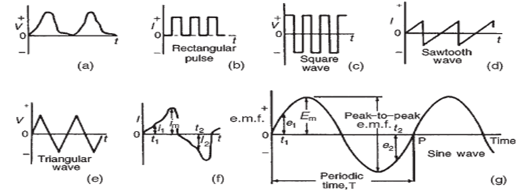
If values of quantities which vary with time t are plotted against time, the resulting graph is called a waveform. A waveform can be unidirectional as shown in (a) and (b) and can be alternating as shown in (c) to (g).  

Unidirectional waveforms as the name implies, travel in one direction (i.e. it doesn’t cross the horizontal axis to the negative side) while the alternating waveforms travels by changing their directions periodically (i.e. alternates) between the positive vertical axis and the negative vertical axis.

A waveform of the type shown in (g) is called a sine wave (or sinusoidal waveform). It is the shape of the waveform of e.m.f. (defined as the electric potential produced by either an electrochemical cell or by changing the magnetic field) produced by an alternator and hence it is the form of mains electricity supply or electricity supply used in various homes, industries and commercial places

Properties of waveforms

The following are the properties of waveforms: time-period (or period or periodic time), frequency, amplitude, wavelength, speed and phase

Time-period

One complete series of values is called a cycle (i.e. from O to P in g) The time taken for an alternating quantity to complete one cycle is called the period or the time-period (T) of the waveform and is measured in seconds (s).

Frequency

The number of cycles completed in one second is called the frequency (f) of the supply and is measured in hertz (Hz). The frequency of the electricity supply varies from region to region or sometimes country to country. For example, the supply frequency in Nigeria and the UK is 50 Hz while the frequency in the US is 60 Hz.

Mathematically, the time-period (T) is related to the frequency (f) by the equation:

T = ¹/_f  or f = ¹/_T

Examples

1. Calculate the time-period for each of the following frequencies: (a) 60 Hz (b) 10 kHz

Solution

(a) Time period (T) = ¹/_f = ¹/₆₀ = 0.0167s

(b) Time period (T) = ¹/_f = ¹/₁₀₀₀₀ = 100μs

2. Calculate the frequency for each of the following time-periods: (a) 2 ms (b) 8 μs

Solution

(a) Frequency  (f) = ¹/_T = ¹/_(2×10^-3) = 500Hz

(b) Frequency  (f) = ¹/_T = ¹/_(8×10^-6) = 125kHz

3. If an alternating voltage completes 6 cycles in 10ms, determine the frequency.

Solution

Frequency (f) is the number of cycles completed in one second. That means the frequency is the ratio of number of completed cycles to time. Therefore, 

 f = ^{number of completed cycles} / _time = ⁶ / _(10×10^-3) = 600Hz or 0.6kHz

4. An alternating current takes 30 μs to complete 3 cycles, what is its time-period?

Solution

Time-period (T) is the time taken to complete one cycle. That means the time-period is the ratio of time to number of cycles completed. Therefore,  

Time period = ^Time / _{number of completed cycles} = ^30×10-6 / ₃ = 10 μs

Amplitude

Amplitude of a waveform is the maximum vertical distance measured from zero (i.e. from the x-axis). Its unit depends on the quantity being considered. If current is being considered, its unit is ampere (A) and if voltage is being considered, the unit is volt (V).

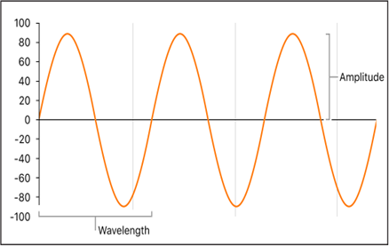
Wavelength

The wavelength of a waveform is defined as the distance between the recurring cycles of a waveform of a given frequency. The higher the frequency, the shorter the wavelength. It is represented as λ and measured in metres (m).

Speed

This is the distance travelled by a waveform per unit time. It is also called wave velocity. It is measured in metres per second (m/s). It is represented as “c”. Speed of a waveform is related mathematically to both frequency and wavelength as:

c = f ג

Phase

Phase is used to state the timing of a point in a waveform or to compare timing between waveforms. It is measured in degrees (from 0⁰ to 360⁰) or radians ( rad).

Peak value

Prior to our discussion of peak values, there is the need to discuss some related terms like instantaneous values and average or mean values, when talking about alternating waveforms or alternating quantities.

Instantaneous value

Instantaneous values are the values of the alternating quantities at any instant of time. These can be seen on the graphs

Average value

Assuming an alternating quantity, the average or mean value of such quantity is the average value measured over a half-cycle. The complete cycle is not considered because for every value in the positive half cycle, there is a corresponding value in the negative half cycle. Hence, the average or mean value is zero over a complete cycle.

With respect to current waveform, the average value of the alternating current can be obtained by considering a half circle divided into a number of parts with equal intervals of time. Then, corresponding current can be obtained for their mid ordinate. The average current (I_av) is thus given as:

I_av = ^{( i₁ + i₂ + i₃ +…i_n)} / _n  

Where i_n is the instantaneous current at any instant as shown below and  is the number of parts the half cycle is divided into.

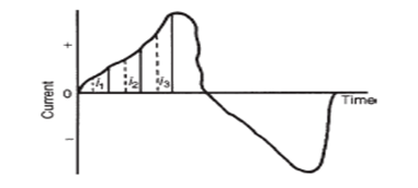
Alternatively,  Average or mean value = ^{area under the curve} / _{base length}

Average values of voltage, current and e.m.f. are represented by V_av, I_av and E_av  respectively etc.

After discussing the instantaneous values and average or mean values, the peak value (or maximum value) of a waveform is the highest or the lowest vertical point of the waveform.

There are two peak points based on this definition i.e. the positive peak point and the negative peak point. The positive peak point is the highest point of the waveform along the positive axis of the e.m.f., while the negative peak point is the lowest point of the waveform along the negative axis of the e.m.f.. The distance between the two peak points is known as the Peak-to-peak e.m.f.

Capital letters with subscript m like I_m, V_m, E_m etc. are used to represent the peak values of current, voltage, e.m.f.

For a sine wave: average value = 0.637 × maximum value

R.M.S.

R.M.S. is an acronym for the root mean square. The root mean square value of an alternating current is the current that yields the same heating effect as an equivalent direct current. Unless otherwise stated, anytime an alternating quantity is given, we assume it is the r.m.s. value. For instance, the mains voltage supply in the UK is 230V which means 230V r.m.s..

Capital letters of respective alternating quantities are used to represent the corresponding r.m.s values i.e. V is used for r.m.s. voltage, I is used for r.m.s. current and E is for r.m.s. e.m.f.  

Considering the waveform divided into a number of segments as shown above, 

The r.m.s. value of the current (I) is:

I = ^{√(i₁2 + i₂2 + i₃2 + …i_n2)} / _n  

Where i is the value of the current at any instant which is called instantaneous current and n is the number of segments the waveform is divided into.

it is clear that the r.m.s. value is the root of the mean of the squares of currents at any instant of time (instantaneous currents) hence, the name root mean square. 

r.m.s. value = 0.707× maximum value 

Form factor = ^r.m.s / _{average value} = ^{0.707 x max value} / _{0.637 x max value} = 1.11 ( for a sine wave)

Peak factor = ^{maximum value} / _{r.m.s value} = ¹ / _0.707 = 1.412 ( for a sine wave)

 

---

Interested in our Electrical Engineering Courses?

At iLearn Engineering^®, we offer a diverse range of online accredited electrical engineering courses and qualifications to cater to different academic and career goals. Our courses are available in varying credit values and levels, ranging from 40 credit Engineering Diplomas to a 360 credit International Graduate Diploma.

Short Courses (40 Credits)

A selection of our more popular 40 credit electrical diplomas…

Diploma in Electrical and Electronic Engineering

Diploma in Electrical Technology

Diploma in Electronics

Diploma in Renewable Energy (Electrical)

First Year of Undergraduate (Level 4 – 120 Credits)

Higher International Certificate in Electrical and Electronic Engineering

First Two Years of Undergraduate (Level 5 – 240 Credits)

Higher International Diploma in Electrical and Electronic Engineering.

Degree equivalent Graduate Diploma (Level 6 – 360 Credits)

 International Graduate Diploma in Electrical and Electronic Engineering

All Electrical and Electronic Courses

You can read more about our selection of accredited online Electrical and Electronic Engineering courses here.

Complete Engineering Course Catalogue (all courses)

Alternatively, you can view all our online engineering courses here.