How can we solve practical problems involving distance and velocity?

In our last article we looked at SI units, what they are and why we use them, giving us a solid introduction to Engineering Science.  In this article, we’re going to see how we can solve some practical problems with engineering.

Introduction to definitions

Before we dive in, it’s useful to introduce some definitions.  In engineering, words such as distance and velocity are associated with mathematical quantities and have strict definitions.  The mathematical quantities used to describe object motion are divided into two categories.  The quantity is either a vector or a scalar and have distinct definitions:

• Scalars are quantities fully described by a magnitude (numerical value) alone.
• Vectors are quantities fully described by both magnitude and direction.

Distance is a scalar quantity that refers to “how much ground an object has covered” during its motion.  Velocity is a vector quantity, and is direction aware.  So, it’s not enough to say an object has a velocity of 55 m/s; we have to also include direction information.

Constant Acceleration Equations

An object with an initial velocity of u is moving in a straight line with constant acceleration a. The equations below connect the final velocity v and displacement s in a given time t.

s = ½(u + v)tv = u + ats = ut + ½ at2s = vt – 1/2 at2v2 = u2 + 2as

s = distance or displacement (m)u = initial velocity (m/s)v = final velocity (m/s)a = acceleration (m/s2)

It’s worth noting that these equations can only be used if the acceleration is constant; for example, in a free fall situation, the acceleration is fixed due to gravity.  The equations are often referred to as SUVAT equations.

Let’s have a look at some examples to see how we can use these equations.  Imagine a vehicle moving in a straight line from O to A, with a constant acceleration of 2m/s².  Its velocity at A is 30m/s, and it takes 15 seconds to travel from O to A.  We’re going to find the vehicle’s velocity at O.

So, the known quantities we have are:

• a = 2m/s²
• v = 30 m/s
• t = 15s

To find u, the initial velocity at O, we use v = u + at.  Which is 30 = u+(2)(15) and gives us 0ms.  Now we’re going to find the distance between O and A, and use the equation s = ut + 1/2 at2.  So, s = 0 + ½(2)(15), which gives us 225 m.

We’ll look at another example.  An object is projected vertically upwards with a velocity of 20 m/s.  The point of projection is on the edge of a deep (30 m) hole, so that the object will continue descending to the bottom of the hole.  We’ll assume gravity, g, is 9.81 m/s².  We’re going to find:

1. The maximum height reached.
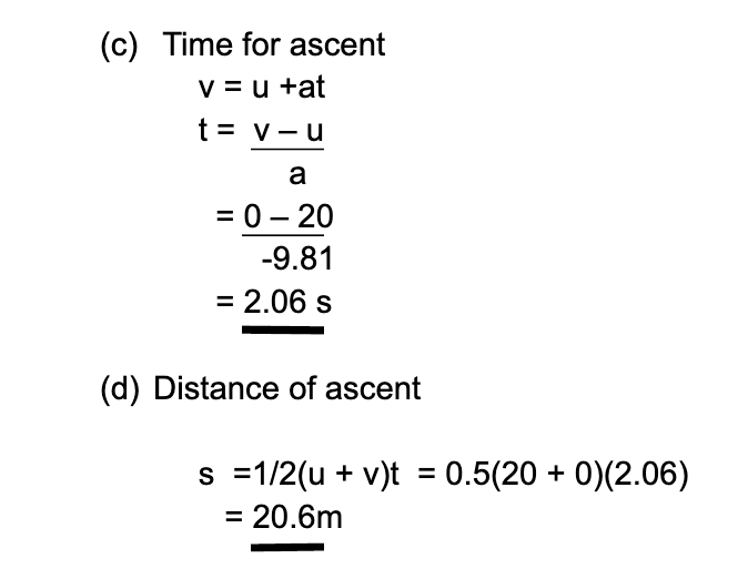
2. The time taken to reach the maximum height.
3. The total time of the flight.
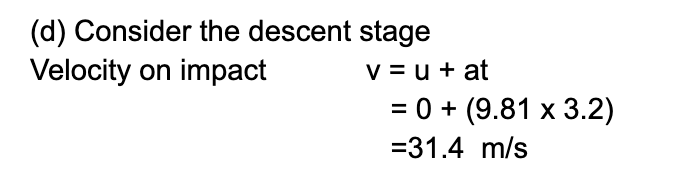
4. The velocity with which the object hits the bottom of the hole.

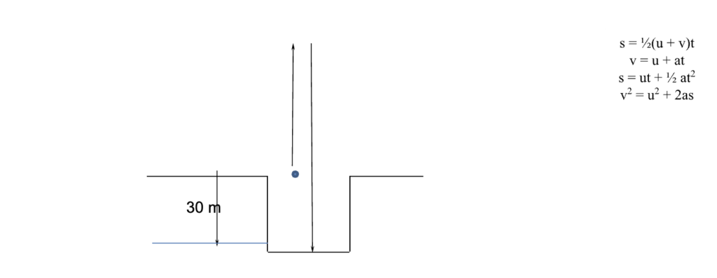
It makes sense to split the motion into ascent and descent.  For the ascent: u=20 m/s, u=0, a=-g

It also makes sense to split the motion into ascent and descent.  For the ascent: u=20 m/s, u=0, a=-g

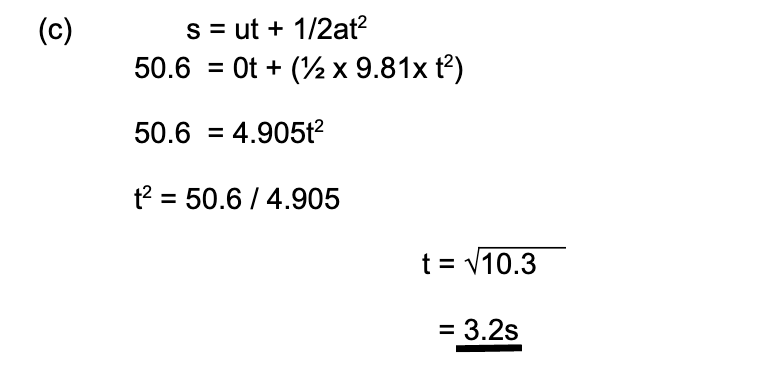
For the descent: u = 0, s = 20.60 + 30 = 50.6m

So, the total time of flight = time ascent + time descent  = 2.06 + 3.2 = 5.3 s

In our next article, we’re going to look at how we can use engineering concepts to solve practical problems, so make sure you keep an eye out for it.

Interested in our courses?

You can read more about our selection of accredited online mechanical, electrical, civil and aerospace engineering courses here.

Check out individual courses pages below:

Diploma in Electrical and Electronic Engineering

Higher International Certificate in Electrical and Electronic Engineering

Diploma in Electrical Technology

Diploma in Electronics

Diploma in Renewable Energy (Electrical)

Higher International Diploma in Electrical and Electronic Engineering

Diploma in Civil Engineering

Diploma in Renewable Energy

Diploma in Material Science

Diploma in Sustainable Construction

Diploma in Structural Engineering

Diploma in Building and Construction Engineering

Diploma in Thermofluids

Higher International Certificate in Civil Engineering

Higher International Diploma in Civil Engineering 

Diploma in Aircraft Design

Diploma in Aerospace Structures

Diploma in Principles of Flight

Diploma in Aerodynamics, Propulsion and Space

Higher International Diploma in Mechanical Engineering

Higher International Certificate in Mechanical Engineering

Diploma in Mechanical Engineering

Diploma in Mechanical Technology

Alternatively, you can view all our online engineering courses here.